Scaling Like a Boss with Presto
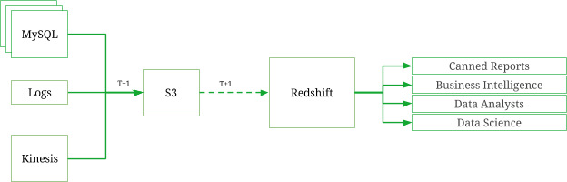
A year ago, the data volumes at Grab were much lower than the volume we currently use for data-driven analytics. We had a simple and robust infrastructure in place to gather, process and store data to be consumed by numerous downstream applications, while supporting the requirements for data science and analytics.
Our analytics data store, Amazon Redshift, was the primary storage machine for all historical data, and was in a comfortable space to handle the expected growth. Data was collected from disparate sources and processed in a daily batch window; and was available to the users before the start of the day. The data stores were well-designed to benefit from the distributed columnar architecture of Redshift, and could handle strenuous SQL workloads required to arrive at insights to support out business requirements.
While we were confident in handling the growth in data, what really got challenging was to cater to the growing number of users, reports, dashboards and applications that accessed the datastore. Over time, the workloads grew in significant numbers, and it was getting harder to keep up with the expectations of returning results within required timelines. The workloads are peaky with Mondays being the most demanding of all. Our Redshift cluster would struggle to handle the workloads, often leading to really long wait times, occasional failures and connection timeouts. The limited workload management capabilities of Redshift also added to the woes.
In response to these issues, we started conceptualising an alternate architecture for analytics, which could meet our main requirements:
- The ability to scale and to meet the demands of our peaky workload patterns
- Provide capabilities to isolate different types of workloads
- To support future requirements of increasing data processing velocity and reducing time to insight
So We Built the Data Lake
We began our efforts to overcome the challenges in our analytics infrastructure by building out our Data Lake. It presented an opportunity to decouple our data storage from our computational modules while providing reliability, robustness, scalability and data consistency. To this effect, we started replicating our existing data stores to Amazon’s Simple Storage Service (S3), a platform proven for its high reliability, and widely used by data-driven companies as part of their analytics infrastructure.
The data lake design was primarily driven by understanding the expected usage patterns, and the considerations around the tools and technologies allowing the users to effectively explore the datasets in the data lake. The design decisions were also based on the data pipelines that would collect the data and the common data transformations to shape and prepare the data for analysis.
The outcome of all those considerations were:
- All large datasets were sharded/partitioned based on the timestamps, as most of the data analysis involved a specific time range and it gave an almost even distribution of data over a length of time. The granularity was at an hour, since we designed the data pipelines to perform hourly incremental processing. We followed the prescribed technique to build the S3 keys for the partitions, which is using the year, month, day and hour prefixes that are known to work well with big data tools such as Hive and Spark.
- Data was stored as AVRO and compressed for storage optimisations. We considered several of the available storage formats - ORC, Parquet, RC File, but AVRO emerged as the elected winner mainly due to its compatibility with Redshift. One of the focus points during the design was to offload some of the heavy workloads run on Redshift to the data lake and have the processed data copied to Redshift.
- We relied on Spark to power our data pipelines and handle the important transformations. We implemented a generic framework to handle different data collection methodologies from our primary data sources - MySQL and Amazon Kinesis. The existing workloads in Redshift written in SQL were easy enough to be replicated on Spark SQL with minimal syntax changes. For everything else we relied on the Spark data frame API.
- The data pipelines were designed to perform, what we started to term as RDP, Recursive Data Processing. While majority of the data sets handled were immutable such as driver states, availability and location, payment transactions, fare requests and more, we still had to deal with the mutable nature of our most important datasets - bookings and candidates. The life cycle of a passenger booking request goes through several states from the starting point of when the booking request was made, through the assignment of the driver, to the length of the ride until completion. Since we collected data at hourly intervals we had to reprocess the bookings previously collected and update the records in the data lake. We performed this recursively until the final state of the data was captured. Updating data stored as files in the data lake is an expensive affair and our strategy to partition, format and compress the data made it achievable using Spark jobs.
- RDP posed another interesting challenge. Most of the data transformation workloads, for example - denormalising the data from multiple sources, required the availability of the individual hourly datasets before the workloads were executed. Managing the workloads to orchestrate complex dependencies at hourly frequencies required a suitable scheduling tool. We were faced with the classic question - to adapt, or to build our own? We chose to build a scheduler that fit the bill.
Once we had the foundational blocks defined and the core components in place, the actual effort in building the data lake was relatively low and the important datasets were available to the users for exploration and analytics in a matter of few days to weeks. Also, we were able to offload some of the workload from Redshift to the data lake with EMR + Spark as the platform and computational engine respectively. However, retrospectively speaking, what we didn’t take into account was the adaptability of the data lake and the fact that majority of our data consumers had become more comfortable in using a SQL-based data platform such as Redshift for their day-to-day use of the data stores. Working with the data using tools such as Spark and Zeppelin involved a larger learning curve and was limited to the skill sets of the data science teams.
And more importantly, we were yet to tackle our most burning challenge, which was to handle the high workload volumes and data requests that was one of our primary goals when we started. We aimed to resolve some of those issues by offloading the heavy workloads from Redshift to the data lake, but the impact was minimal and it was time to take the next steps. It was time to presto.
Gusto with Presto
SQL on Hadoop has been an evolving domain, and is advancing at a fast pace matching that of other big data frameworks. A lot of commercial distributions of the Hadoop platform have taken keen interest in providing SQL capabilities as part of their ecosystem offerings. Impala, Stinger, Drill appear to be the frontrunners, but being on the AWS EMR stack, we looked at Presto as our SQL engine over the data lake in S3.
The very first thing we learnt was the lack of support for the AVRO format in Presto. However, that seemed to be the only setback as it was fairly straightforward to adapt Parquet as the data storage format instead of AVRO. Presto had excellent support for Hive metastore, and our data lake design principles were a perfect fit for that. AWS EMR had a fairly recent version of Presto when we started (they have upgraded to more recent versions since). Presto supports ANSI SQL. While the syntax was slightly different to Redshift, we had no problems to adapt and work with that. Most importantly, our performance benchmarks showed results that were much better than anticipated. A lot of online blogs and articles about Presto always tend to benchmark its performance against Hive which frankly doesn’t provide any insights on how well Presto can perform. What we were more interested in was to compare the performance of Presto over Redshift, since we were aiming to offload the Redshift workloads to Presto. Again, this might not be a fair enough comparison since Redshift can be blazingly fast with the right distribution and sort keys in place, and well written SQL queries. But we still aimed to hit at-least 50-60% of the performance numbers with Presto as compared to Redshift, and were able to achieve it in a lot of scenarios. Use cases where the SQL only required a few days of data (which was mostly what the canned reports needed), due to the partitions in the data, Presto performed as well as (if not better than) Redshift. Full table scans involving distribution and sort keys in Redshift were a lot faster than Presto for sure, but that was only needed as part of ad-hoc queries that were relatively rare.
We compared the query performance for different types of workloads:
- A. Aggregation of data on the entire table (2 Billion records)
- Sort key column used in Redshift
- B. Aggregation of data with a specific data range (1 week)
- Partitioning fields used in Presto
- C. Single record fetch
- D. Complex SQL query with join between a large table (with date range) and multiple small tables
- E. Complex SQL query with join between two large tables (with date range) and multiple small tables
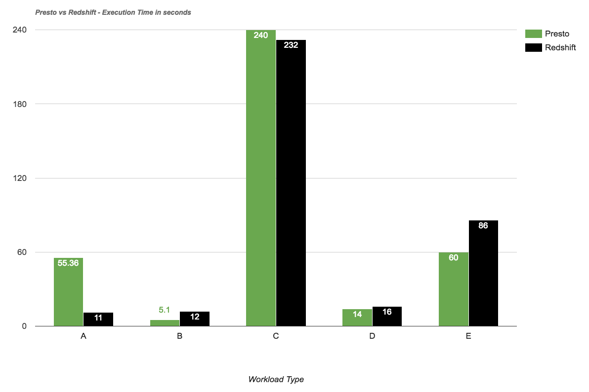
Notes on the performance comparison:
- The Presto and Redshift clusters had similar configurations
- No other workloads were being executed when the performance tests were run.
Although Presto could not exceed the query performance of Redshift in all scenarios, we could divide the workloads across different Presto clusters while maintaining a single underlying storage layer. We wanted to move away from a monolithic multi-tenant to a completely different approach of shared-data multi-cluster architecture, with each cluster catering to a specific application or a type of usage or a set of users. Hosting Presto on EMR provided us with the flexibility to spin up new clusters in a matter of minutes, or scale existing clusters during peak loads.
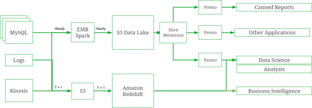
With the introduction of Presto to our analytics stack, the architecture now stands as depicted:
From an implementation point of view, each Presto cluster would connect to a common Hive metastore built on RDS. The Hive metastore provided the abstraction over the Parquet datasets stored in the data lake. Parquet is the next best known storage format suited for Presto after ORC, both of which are columnar stores with similar capabilities. A common metastore meant that we only had to create a Hive external table on the datasets in S3 and register the partitions once, and all the individual presto clusters would have the data available for querying. This was both convenient and provided an excellent level of availability and recovery. If any of the cluster went down, we would failover to a standby Presto cluster in a jiffy, and scale it for production use. That way we could ensure business continuity and minimal downtime and impact on the performance of the applications dependant on Presto.
The migration of workloads and canned SQL queries from Redshift to Presto was time consuming, but all in all, fairly straightforward. We built custom UDFs for Presto to simplify the process of migration, and extended the support on SQL functions available to the users. We learnt extensively about writing optimised queries for Presto along the way. There were a few basic rules of thumb listed below, which helped us achieve the performance targets we were hoping for.
- Always rely on the time-based partition columns whenever querying large datasets. Using the partition columns restricts the amount of data being read from S3 by Presto.
- When joining multiple tables, ordering the join sequences based on the size of the table (from largest to the smallest) provided significant performance benefits and also helped avoid skewness in the data that usually leads to “exceeds memory limit” exceptions on Presto.
- Anything other than equijoin conditions would cause the queries to be extremely slow. We recommend avoiding non equijoin conditions as part of the ON clause, and instead apply them as a filter within the WHERE clause wherever possible.
- Sorting of data using
ORDER BYclauses must be avoided, especially when the resulting dataset is large. - If a query is being filtered to retrieve specific partitions, use of SQL functions on the partitioning columns as part of the filtering condition leads to a really long PLANNING phase, during which Presto is trying to figure out the partitions that need to be read from the source tables. The partition column must be used directly to avoid this effect.
Back on the Highway
It has been a few months since we have adopted Presto as an integral part of our analytics infrastructure, and we have seen excellent results so far. On an average we cater to 1500 - 2000 canned report requests a day at Grab, and support ad-hoc/interactive query requirements which would most likely double those numbers. We have been tracking the performance of our analytics infrastructure since last year (during the early signs of the troubles). We hit the peak just before we deployed Presto into our production systems, and the migration has since helped us achieve a 400% improvement in our 90th percentile numbers. The average execution times of queries have also improved significantly, and we have successfully eliminated the high wait times that were associated with the Redshift workload manager during periods with large numbers of concurrent requests.
Conclusion
Adding Presto to our stack has give us the boost we needed to scale and meet the growing requirements for analytics. We have future-proofed our infrastructure by building the data lake, and made it easier to evaluate and adapt new technologies in the big data space. We hope this article has given you insights in Grab’s analytics infrastructure. We would love to hear your thoughts or your experience, so please do leave a note in the comments below.
Many thanks to Edwin Law who reviewed drafts and waited patiently for it to be published.