Introduction

In 2022, Grab achieved self-sufficiency in its Geo services. As part of this transition, one crucial step was moving towards using an internally-developed map tailored specifically to the market in which Grab operates. Now that we have full control over the map layer, we can add more data to it or improve it according to the needs of the services running on top. One key aspect that this transition unlocked for us was the possibility of creating hyperlocal data at map level.

For instance, by determining the country to which a road belongs, we can now automatically infer the official language of that country and display the street name in that language. In another example, knowing the country for a specific road, we can automatically infer the driving side (left-handed or right-handed) leading to an improved navigation experience. Furthermore, this capability also enables us to efficiently handle various scenarios. For example, if we know that a road is part of a gated community, an area where our driver partners face restricted access, we can prevent the transit through that area.

These are just some examples of the possibilities from having full control over the map layer. By having an internal map, we can align our maps with specific markets and provide better experiences for our driver-partners and customers.

Background

For all these to be possible, we first needed to localise the roads inside the map. Our goal was to include hyperlocal data into the map, which refers to data that is specific to a certain area, such as a country, city, or even a smaller part of the city like a gated community. At the same time, we aimed to deliver our map with a high cadence, thus, we needed to find the right way to process this large amount of data while continuing to create maps in a cost-effective manner.

Solution

In the following sections of this article, we will use an extract from the Southeast Asia map to provide visual representations of the concepts discussed.

In Figure 1, Image 1 shows a visualisation of the road network, the roads belonging to this area. The coloured lines in Image 2 represent the borders identifying the countries in the same area. Overlapping the information from Image 1 and Image 2, we can extrapolate and say that the entire surface included in a certain border could have the same set of common properties as shown in Image 3. In Image 4, we then proceed with adding localised roads for each area.

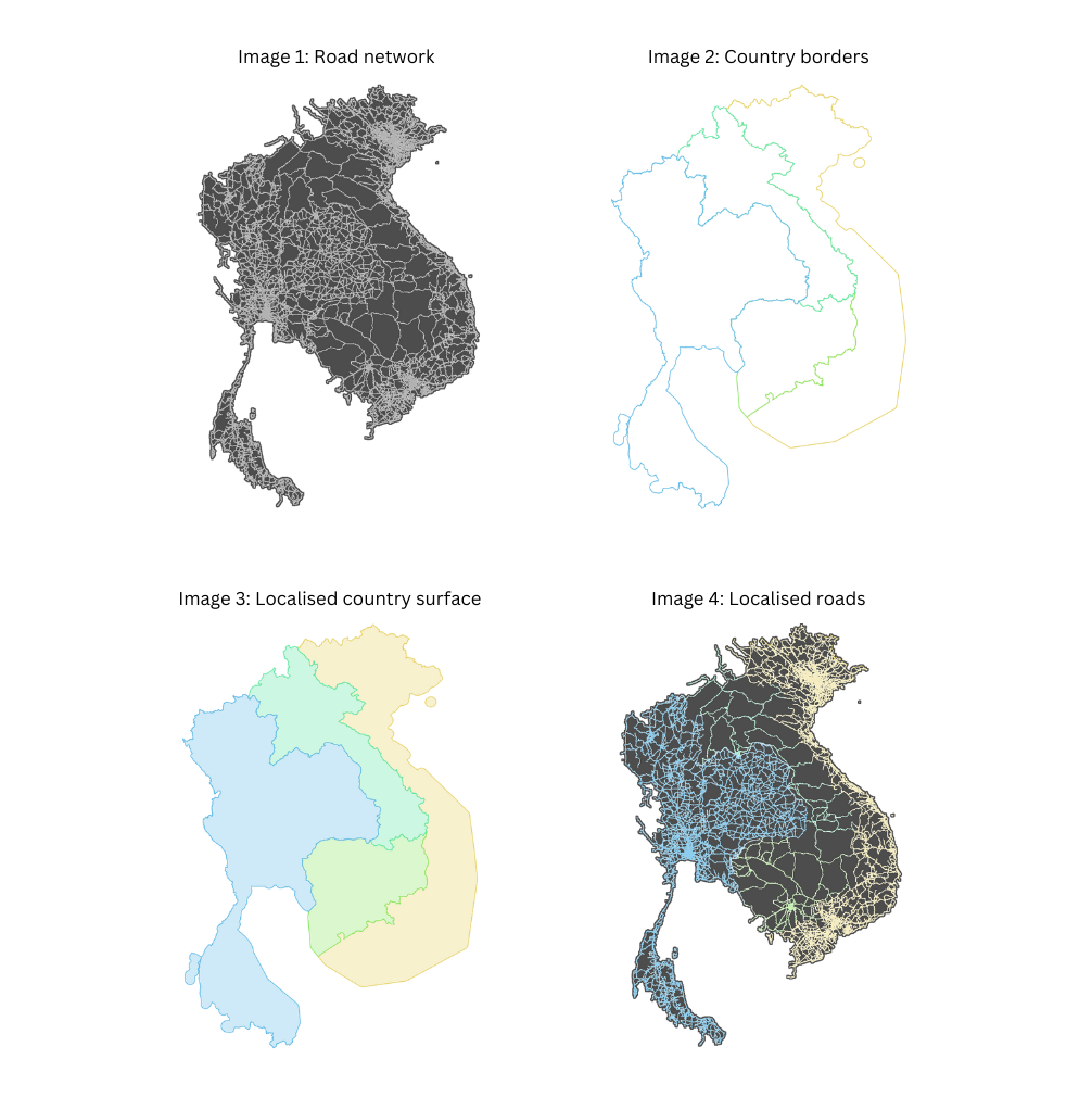
For this to be possible, we have to find a way to localise each road and identify its associated country. Once this localisation process is complete, we can replicate all this information specific to a given border onto each individual road. This information includes details such as the country name, driving side, and official language. We can go even further and infer more information, and add hyperlocal data. For example, in Vietnam, we can automatically prevent motorcycle access on the motorways.

Assigning each road on the map to a specific area, such as a country, service area, or subdivision, presents a complex task. So, how can we efficiently accomplish this?

Implementation

The most straightforward approach would be to test the inclusion of each road into each area boundary, but that is easier said than done. With close to 30 million road segments in the Southeast Asia map and over 10 thousand areas, the computational cost of determining inclusion or intersection between a polyline and a polygon is expensive.

Our solution to this challenge involves replacing the expensive yet precise operation with a decent approximation. We introduce a proxy entity, the geohash, and we use it to approximate the areas and also to localise the roads.

We replace the geometrical inclusion with a series of simpler and less expensive operations. First, we conduct an inexpensive precomputation where we identify all the geohases that belong to a certain area or within a defined border. We then identify the geohashes to which the roads belong to. Finally, we use these precomputed values to assign roads to their respective areas. This process is also computationally inexpensive.

Given the large area we process, we leverage big data techniques to distribute the execution across multiple nodes and thus speed up the operation. We want to deliver the map daily and this is one of the many operations that are part of the map-making process.

What is a geohash?

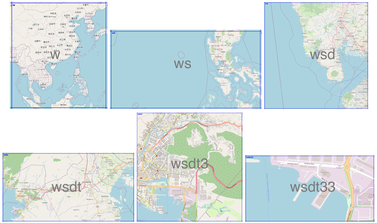
To further understand our implementation we will first explain the geohash concept. A geohash is a unique identifier of a specific region on the Earth. The basic idea is that the Earth is divided into regions of user-defined size and each region is assigned a unique id, which is known as its geohash. For a given location on earth, the geohash algorithm converts its latitude and longitude into a string.

Geohashes uses a Base-32 alphabet encoding system comprising characters ranging from 0 to 9 and A to Z, excluding “A”, “I”, “L” and “O”. Imagine dividing the world into a grid with 32 cells. The first character in a geohash identifies the initial location of one of these 32 cells. Each of these cells are then further subdivided into 32 smaller cells.This subdivision process continues and refines to specific areas in the world. Adding characters to the geohash sub-divides a cell, effectively zooming in to a more detailed area.

The precision factor of the geohash determines the size of the cell. For instance, a precision factor of one creates a cell 5,000 km high and 5,000 km wide. A precision factor of six creates a cell 0.61km high and 1.22 km wide. Furthermore, a precision factor of nine creates a cell 4.77 m high and 4.77 m wide. It is important to note that cells are not always square and can have varying dimensions.

In Figure 2, we have exemplified a geohash 6 grid and its code is wsdt33.

Using less expensive operations

Calculating the inclusion of the roads inside a certain border is an expensive operation. However, quantifying the exact expense is challenging as it depends on several factors. One factor is the complexity of the border. Borders are usually irregular and very detailed, as they need to correctly reflect the actual border. The complexity of the road geometry is another factor that plays an important role as roads are not always straight lines.

Since this operation is expensive both in terms of cloud cost and time to run, we need to identify a cheaper and faster way that would yield similar results. Knowing that the complexity of the border lines is the cause of the problem, we tried using a different alternative, a rectangle. Calculating the inclusion of a polyline inside a rectangle is a cheaper operation.

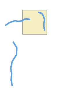
So we transformed this large, one step operation, where we test each road segment for inclusion in a border, into a series of smaller operations where we perform the following steps:

1. Identify all the geohashes that are part of a certain area or belong to a certain border. In this process we include additional areas to make sure that we cover the entire surface inside the border.
2. For each road segment, we identify the list of geohashes that it belongs to. A road, depending on its length or depending on its shape, might belong to multiple geohashes.

In Figure 5, we identify that the road belongs to two geohashes and that the two geohashes are part of the border we use.

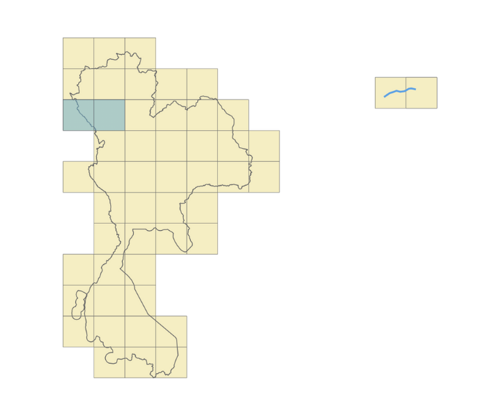
Now, all we need to do is join the two data sets together. This kind of operation is a great candidate for a big data approach, as it allows us to run it in parallel and speed up the processing time.

Precision tradeoff

We mentioned earlier that, for the sake of argument, we replace precision with a decent approximation. Let’s now delve into the real tradeoff by adopting this approach.

The first thing that stands out with this approach is that we traded precision for cost. We are able to reduce the cost as this approach uses less hardware resources and computation time. However, this reduction in precision suffers, particularly for roads located near the borders as they might be wrongly classified.

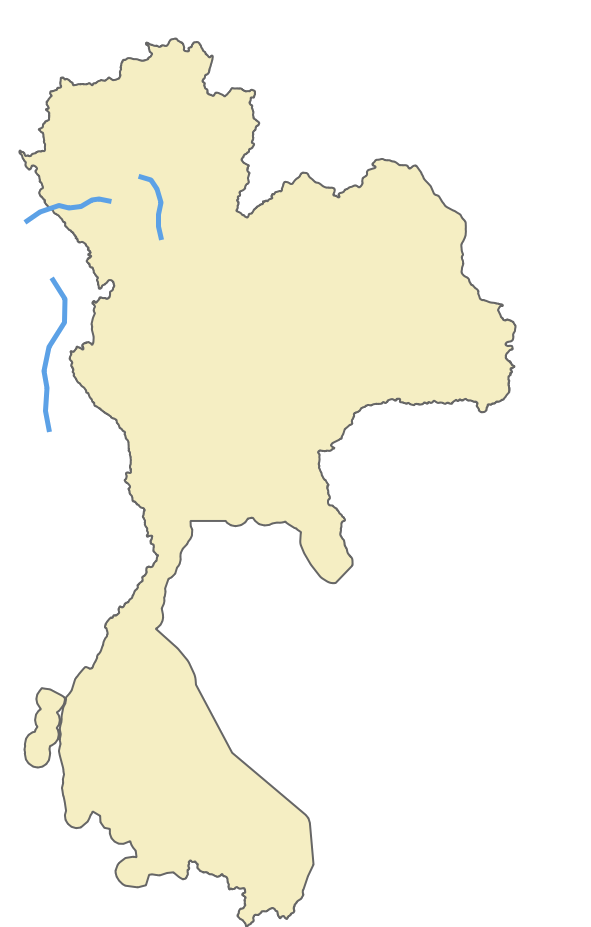
Going back to the initial example, let’s take the case of the external road, on the left side of the area. As you can see in Figure 6, it is clear that the road does not belong to our border. But when we apply the geohash approach it gets included into the middle geohash.

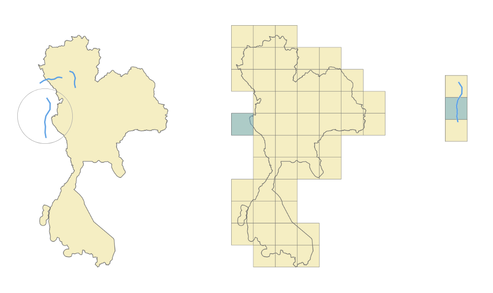
Given that just a small part of the geohash falls inside the border, the entire geohash will be classified as belonging to that area, and, as a consequence, the road that belongs to that geohash will be wrongly localised and we’ll end up adding the wrong localisation information to that road. This is clearly a consequence of the precision tradeoff. So, how can we solve this?

Geohash precision

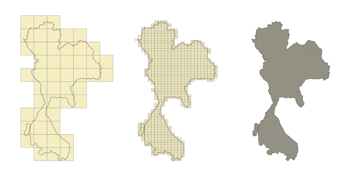
One option is to increase the geohash precision. By using smaller and smaller geohashes, we can better reflect the actual area. As we go deeper and we further split the geohash, we can accurately follow the border. However, a high geohash precision also equates to a computationally intensive operation bringing us back to our initial situation. Therefore, it is crucial to find the right balance between the geohash size and the complexity of operations.

Geohash coverage percentage

To find a balance between precision and data loss, we looked into calculating the geohash coverage percentage. For example, in Figure 8, the blue geohash is entirely within the border. Here we can say that it has a 100% geohash coverage.

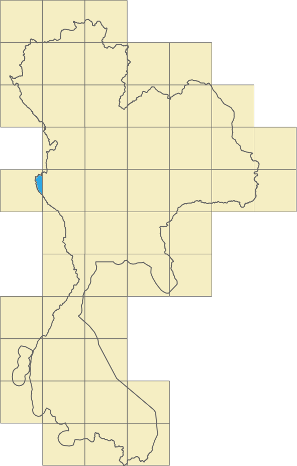
However, take for example the geohash in Figure 9. It touches the border and has only around 80% of its surface inside the area. Given that most of its surface is within the border, we still can say that it belongs to the area.

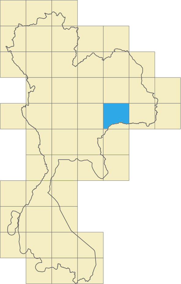
Let’s look at another example. In Figure 10, only a small part of the geohash is within the border. We can say that the geohash coverage percentage here is around 5%. For these cases, it becomes difficult for us to determine whether the geohash does belong to the area. What would be a good tradeoff in this case?

Border shape

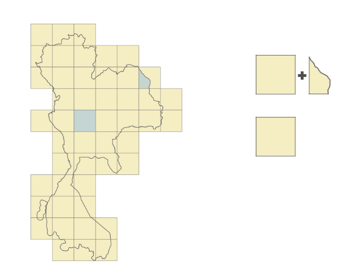
To go one step further, we can consider a mixed solution, where we use the border shape but only for the geohashes touching the border. This would still be an intensive computational operation but the number of roads located in these geohashes will be much smaller, so it is still a gain.

For the geohashes with full coverage inside the area, we’ll use the geohash for the localisation, the simpler operation. For the geohashes that are near the border, we’ll use a different approach. To increase the precision around the borders, we can cut the geohash following the border’s shape. Instead of having a rectangle, we’ll use a more complex shape which is still simpler than the initial border shape.

Result

We began with a simple approach and we enhanced it to improve precision. This also increased the complexity of the operation. We then asked, what are the actual gains? Was it worthwhile to go through all this process? In this section, we put this to the test.

We first created a benchmark by taking a small sample of the data and ran the localisation process on a laptop. The sample comprised approximately 2% of the borders and 0.0014% of the roads. We ran the localisation process using two approaches.

• With the first approach, we calculated the intersection between all the roads and borders. The entire operation took around 38 minutes.
• For the second approach, we optimised the operation using geohashes. In this approach, the runtime was only 78 seconds (1.3 minutes).

However, it is important to note that this is not an apples-to-apples comparison. The operation that we measured was the localisation of the roads but we did not include the border filling operation where we fill the borders with geohashes. This is because this operation does not need to be run every time. It can be run once and reused multiple times.

Though not often required, it is still crucial to understand and consider the operation of precomputing areas and filling borders with geohashes. The precomputation process depends on several factors:

• Number and shape of the borders - The more borders and the more complex the borders are, the longer the operation will take.
• Geohash precision - How accurate do we need our localisation to be? The more accurate it needs to be, the longer it will take.
• Hardware availability

Going back to our hypothesis, although this precomputation might be expensive, it is rarely run as the borders don’t change often and can be triggered only when needed. However, regular computation, where we find the area to which each road belongs to, is often run as the roads change constantly. In our system, we run this localisation for each map processing.

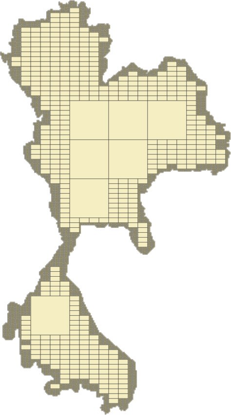
We can also further optimise this process by applying the opposite approach. Geohashes that have full coverage inside a border can be merged together into larger geohashes thus simplifying the computation inside the border. In the end, we can have a solution that is fully optimised for our needs with the best cost-to-performance ratio.

Conclusion

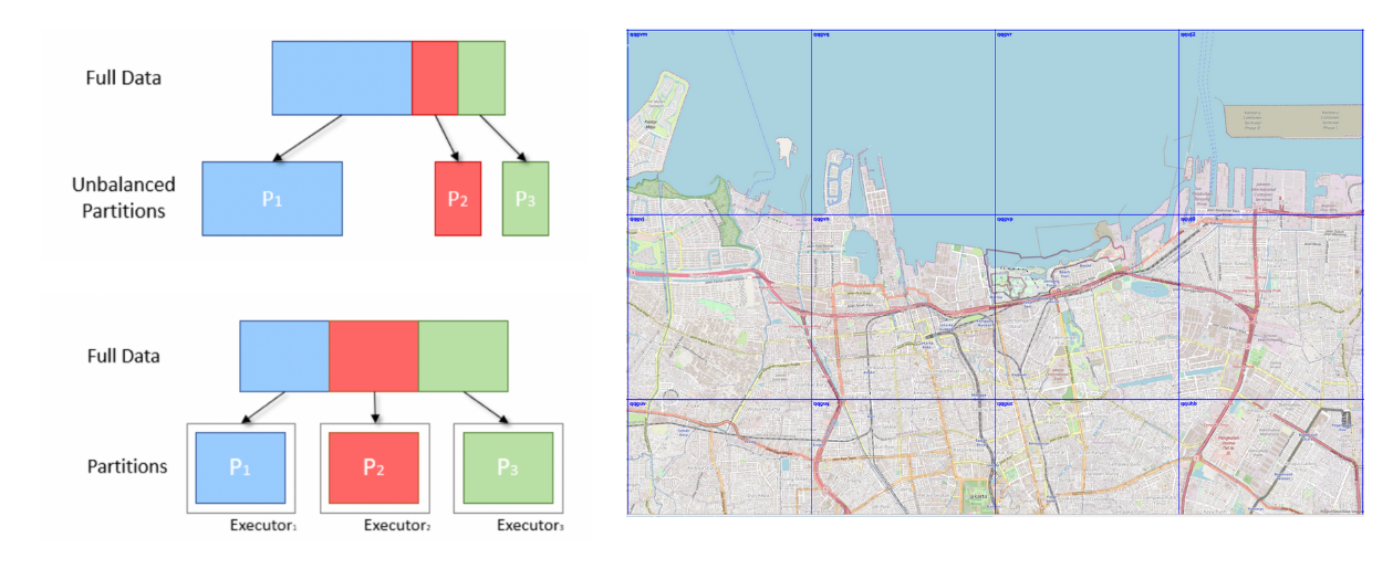
Although geohashes seem to be the right solution for this kind of problem, we also need to monitor their content. One consideration is the road density inside a geohash. For example, a geohash inside a city centre usually has a lot of roads while one in the countryside may have much less. We need to consider this aspect to have a balanced computation operation and take full advantage of the big data approach. In our case, we achieve this balance by considering the number of road kilometres within a geohash.

Additionally, the resources that we choose also matter. To optimise time and cost, we need to find the right balance between the running time and resource cost. As shown in Figure 14, based on a sample data we ran, sometimes, we get the best result when using smaller machines.

The achievements and insights showcased in this article are indebted to the contributions made by Mihai Chintoanu. His expertise and collaborative efforts have profoundly enriched the content and findings presented herein.

Join us

Grab is the leading superapp platform in Southeast Asia, providing everyday services that matter to consumers. More than just a ride-hailing and food delivery app, Grab offers a wide range of on-demand services in the region, including mobility, food, package and grocery delivery services, mobile payments, and financial services across 428 cities in eight countries.

Powered by technology and driven by heart, our mission is to drive Southeast Asia forward by creating economic empowerment for everyone. If this mission speaks to you, join our team today!