
Migrating Counter Service storage: Design choices and learnings
Introduction
Counter Service is used across Grab’s anti-fraud platform to answer time-windowed count questions, such as recent ride requests by a user or failed payment attempts on a card. The service handles tens of thousands of queries per second (QPS) with about a billion requests per day, while maintaining strict requirements around latency and reliability to support real-time fraud rule evaluation.
For most of its life, Counter Service was backed by a wide-column database that served the workload reliably as the service scaled. As part of a broader infrastructure review mandated at an organizational level, our database team evaluated alternatives to this storage that many services relied on, including Counter Service. Based on their assessment, Aerospike emerged as a good fit for our use-case. We also used the migration as an opportunity to decouple storage concerns from business logic, a necessary first step for this migration, and one that would reduce the effort required for future storage changes. As part of the same effort, we revisited the data model and access patterns in detail, which helped us identify and apply several straightforward optimizations.
This post walks through how we did it. What we built on the reader-side to make the migration safe, how we redesigned the writer-side data model around the new backend, and what we ran into during the gradual rollout.
Setting the stage
Counter data is stored in three time granularities: 15-minute, hourly, and daily buckets. A typical read would be along the lines of, “give me the count for key X over the last 90 minutes”, which the service decomposes into the smallest possible set of buckets, one hourly in the middle, a few 15-minute buckets at the edges, fetches them, and sums.
In the original setup, each granularity was stored in a separate table with a composite primary key:
TABLE daily_count (
    key      TEXT,         -- partition key
    day_ts   TIMESTAMP,    -- clustering key
    count    BIGINT,
    PRIMARY KEY (key, day_ts)
);
The clustering column gave us convenient range queries, that is needed for the Counter Service. On the write path, each incoming counter event triggered a read-modify-write, three parallel SELECT across the three tables, an in-memory increment, then a batch write. This produced four network round-trips per event.
As this service is a core part of Grab’s fraud detection ecosystem and handles high query volume, migrating its underlying storage required a careful rollout plan. We had three requirements:
- Ramp traffic to the new backend gradually and roll back at any point with a config change.
- Monitor both the original and new storage paths to verify data integrity before switching over.
- Complete the migration without downtime.
We also wanted the migration machinery to be reusable for future storage changes. The migration is divided into three workstreams, which we’ll walk through below:
- Preparing the reader service.
- Identifying the best integration mechanism for the new storage.
- Updating the writer pipeline.
Reader: Separating the data access layer
The reader is a Rust service. Before any migration work began, the reader’s business logic had tight coupling with the storage layer. Session creation, query building, fan-out orchestration, and the data types those queries returned were all intertwined in a single flat file. The main application state struct (AppState) held a raw database session handle and prepared query references. Every handler, gRPC Remote Procedure Calls (gRPC) or HyperText Transfer Protocol (HTTP), received the bare session as a parameter. Variable names baked the storage technology into the business layer.
This made the storage migration difficult to attempt directly. We couldn’t add a second storage backend without forking the orchestration logic, and we had no way to test the read path in isolation from a real database session. So we did the migration prep in three stages.
Stage 1: Extracting the storage code
The first stage shipped no behavioural change. We deleted the monolithic storage file and split its contents in two:
storage/legacy.rs: wrapped session creation, prepared statements, and query execution behind aLegacyStoragestruct.batch_read_ops.rs: kept only the orchestration logic: time-range splitting, channel-based fan-out, and aggregation.
AppState started holding an Arc<LegacyStorage> instead of a raw session handle. The PreparedQueries struct lost its statements (those moved inside LegacyStorage). We renamed every storage-specific identifier in business code to generic storage_* names.
The result was a hard fence. After Stage 1, the database driver crate was reachable only from inside the storage module. Nothing in the business logic or handlers imported it any more.
Stage 2: The storage facade
With the seam in place, we introduced the actual abstraction. A new storage/ module with mod.rs, legacy.rs, aerospike.rs, and mock_storage.rs as siblings became the only place driver crates were reachable from.
The idiomatic Rust approach would have been a trait with associated types, but our backend selection is runtime (a config string parsed at startup), and associated types propagate upwards through every consumer. The alternative, trait objects with boxed futures adds a heap allocation per query, which we wanted to avoid at our QPS.
We chose a concrete facade with enum dispatch:
struct Storage {
    legacy:    LegacyStorage,
    aerospike: AerospikeStorage,
    mock:      MockStorage,
    settings:  StorageSettings,
}

execute_queries(backend: BackendType, ...) {
    match backend {
        Legacy    => self.legacy.execute(...),
        Aerospike => self.aerospike.execute(...),
        Mock      => self.mock.execute(...),
    }
}
A match statement at the request boundary, which made it easier to reason about and debug. The facade then routes everything to the original backend without the rest of the code knowing or caring.
Each backend’s execute_queries honours the same contract: take a Vec<QueryCandidate> and a HashMap<BatchIndex, Sender<...>>, and emit (index, value, timestamp, granularity) tuples into those channels. The orchestration layer above doesn’t need to know whether a candidate became a paginated row stream or a single batch read with client-side map filtering, both write into the same channels in the same shape.
On top of the facade we layered three config-driven operating modes that map to the migration phases:
- Single: one backend serves the request.
- WithShadow: the primary serves the response; the secondary runs asynchronously in the background for parity comparison.
- WithSplit: a deterministic percentage of traffic is served by each backend. Used for the live cutover.
The mode and traffic percentages are read from a service config, allowing the reader to move from legacy-only to Aerospike-only without code changes. The transition starts in Single(legacy), then shadow reads are enabled with WithShadow(primary=legacy, secondary=aerospike, pct=X). The shadow percentage is gradually ramped from 5% to 20%, 50%, and finally 100%, while parity is verified through metrics. Optionally, the system can then move into WithSplit(primary=legacy, secondary=aerospike, split=X), where live traffic is gradually shifted from the original backend to Aerospike, for example from 5% to 30%, 70%, and then 100%. Once Aerospike is fully validated and serving all traffic, the reader moves to Single(aerospike).
Stage 3: Shadow comparison and metrics
Each storage call carries metadata like backend, role (primary/secondary/shadow), and mode, attached as tags to every metric. When Aerospike was added, existing dashboards showed per-backend breakdowns without changes.
We placed the mode dispatch at the handler level rather than inside the storage layer to validate the full request path, not only the rows returned by storage. This also lets the response return as soon as the primary completes, while the shadow runs as a fire-and-forget background task.
Writer: redesigning the data model
Since the two systems use different storage engines, it wasn’t clear that a one-to-one port of our original schema would work. We tried three approaches.
Approaches 1 and 2: Row-per-bucket
We first tried mirroring our original row-per-bucket model. Approach 1 used Aerospike’s Secondary Index (SI) to recover range queries; approach 2 skipped SI and computed the exact set of primary keys client-side via BatchGet.
Both hit the same wall: Aerospike’s primary index is 64 bytes per record, kept in memory. At billions of records, index memory becomes the constraint. SI added overhead and operational complexity we didn’t need.
Approach 3: Map-based schema
The third approach was structurally different from the first two and was the most compact of the options. Rather than storing one record per bucket, which kept us in the same cardinality regime, we collapsed all bucket counts for a single counter into one record. The values were stored as a sorted map keyed by bucket timestamp:
Set:           helium_hourly
Primary key:   "{counterKey}"
Bins:
   counts: KEY_ORDERED_MAP({
        1773369000000: 1,
        1773372600000: 3,
        1773376200000: 7,
        ...
   })
The map keys are bucket timestamps in milliseconds. The map values are running counts. One record holds the entire time series for one counter at one granularity.
Reads become straightforward: fetch the record, iterate the map, sum the entries within the requested window. Each Get returns a bounded number of map entries (determined by Time To Live (TTL) and bucket size), and client-side filtering of that many entries is negligible.
Writes use MapIncrementOp, an atomic server-side increment of a value at a given map key, creating the entry on first access. Combined with MapRemoveByKeyRangeOp for pruning stale entries, every write is one atomic operation:
ops = [
    MapIncrementOp(counts, bucketTsMs, delta),
    MapRemoveByKeyRangeOp(counts, 0, cutoffMs),
    PutOp(key_bin, counterKey),
]
client.Operate(policy, key, ops)
For TTL management, we couldn’t use Aerospike’s record-level expiry directly. A single record holds many timestamps, so record-level TTL would either keep everything or drop everything. Instead, we prune stale map entries explicitly on every write using MapRemoveByKeyRangeOp. The record-level TTL stays as a safety net for counters that stop receiving writes.
The two backends produce very different network shapes for the same logical query. The original backend returns many small paginated row streams, one per (key, granularity). The server filters by time range using the clustering column. Aerospike returns one batch response with the entire counts map per key, and the client filters the map to the requested range. The reader’s storage layer hides this difference: both paths emit (index, value, timestamp, granularity) tuples into the same per-index channels, and the orchestrator above sums them the same way.
The third approach performed best in testing. By collapsing many bucket records into a single record per counter, we reduced the total record count by more than an order of magnitude, which also reduced primary index memory. It also produced a smaller on-disk footprint, since the long counter key is stored once per record instead of being repeated across every bucket. The schema was chosen to fit the access pattern, with the index and disk savings following naturally.
The pipeline continues writing to the original backend as the primary, while Aerospike is added as a separate asynchronous shadow write behind a deterministic rollout logic. This lets us ramp Aerospike gradually and eventually cut over to it fully.
Reader: How each backend actually serves a query
The two storage backends sit behind the same execute_queries contract on the reader service, but what they do internally for a single batch read looks very different.
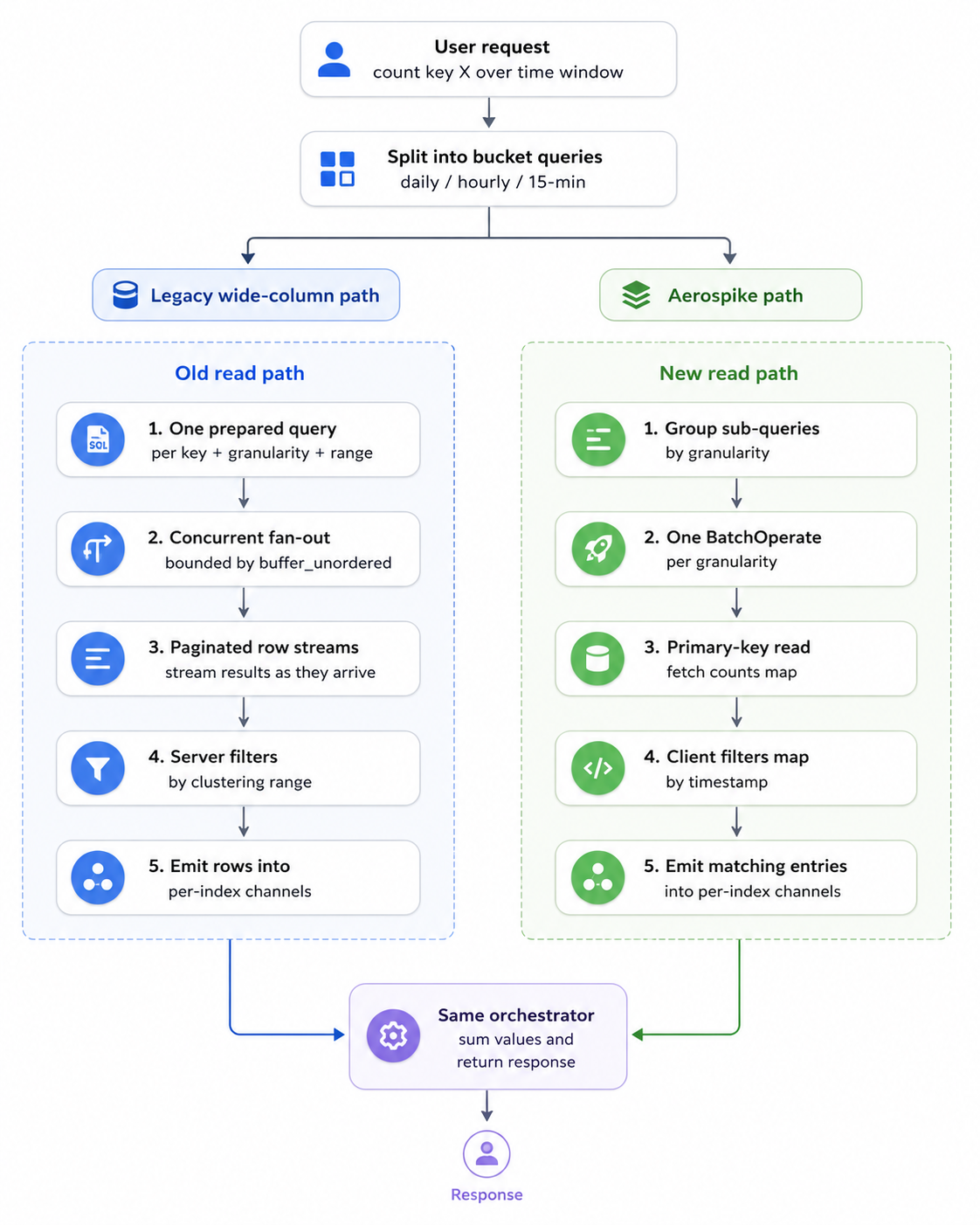
The reader takes a batch of counter queries and decomposes each into one or more sub-queries per granularity (a 90-minute window for instance, becomes one hourly sub-query and two 15-minute sub-queries). In the original backend, each sub-query becomes its own prepared statement bound with (start_ms, end_ms, key), and the storage layer fires all of them concurrently as a stream of futures with buffer_unordered capping in-flight queries to a tuned bound. Each query returns a paginated row iterator, the server uses the clustering column to filter by time range and rows stream through to per-index channels as they arrive. So a single user request can produce many small queries, each a separate network round-trip to the partition master holding key, with results dribbled back over a paginated stream.
On Aerospike, the storage layer first groups all sub-queries by granularity, then issues one BatchOperate per granularity. Each sub-query becomes a single primary-key read against the appropriate set; the server returns the entire counts map for that key in one record. The client iterates the map and emits only the entries whose timestamps fall inside the requested range. This keeps the code simple, and at our map sizes the overhead is negligible. There’s no streaming, a batch read either succeeds or fails as a unit and there are at most three network round-trips per user request, one per granularity, regardless of how many sub-queries there are.
This reflects the different design philosophies of the two systems. Wide-column stores typically expect client-side fan-out for reads, while Aerospike’s batch API is designed for exactly this multi-key pattern.
A few issues with the Aerospike Rust client also surfaced during rollout, as it was less mature than its Go counterpart. For example, when we started, the officially available Rust client was synchronous, so every batch read had to be bridged through tokio::task::spawn_blocking with some amount of custom plumbing. Once the official async client was released, we removed that layer and saw measurable improvements in both p50 and p99 latency. The other issue was Domain Name System (DNS). The client resolved seed hostnames only during initialization and did not re-resolve them when the cluster topology refreshed. As a result, a full staging cluster replacement, with new IPs behind the same hostnames, left the client stuck on the old IPs until restart. We filed the bug upstream, and a fix shipped in a subsequent release. We also reproduced the scenario locally with a Docker-based end-to-end test and ran additional staging drills to confirm recovery before continuing the rollout.
Experiment with indexing
We run Aerospike in its default storage configuration, Hybrid Memory Architecture (HMA), where the primary index sits in Random-Access Memory (RAM) and the data sits on Solid-State Drive (SSD). The other relevant mode keeps both index and data in Dynamic Random-Access Memory (DRAM), which is more expensive and not something that fits our use-case. Even in HMA, the primary index grows linearly with record count. At our scale, that growth was a foreseeable issue.
To raise the memory ceiling, we tried moving the primary index itself from RAM to local Non-Volatile Memory Express (NVMe) while keeping data on SSD. We expected the extra index latency to be invisible within our overall request budget. In practice, we started seeing p99 spikes that did not track overall QPS. Instead, they followed I/O activity on hot keys. We observed that when many concurrent lookups land on the same record, the in-memory index handles them more prudently compared to a disk backed index. Adding more and better nodes improved things slightly but did not mitigate the issue. Consequently, we reverted back to in-memory index with a memory-optimized instance type.
Overall impact
The migration delivered gains across infrastructure, performance, and data footprint. Most of these improvements trace back to the schema redesign like collapsing rows into maps, rather than the database change itself.
The primary index currently uses about 50 GB of the roughly 100 GB usable memory per node. The same dataset is around 1 TB on disk, compared with around 3 TB on the original setup. This is primarily attributed to our adoption of the map-based schema discussed earlier.
In production, p99 read latency was consistently better than the original setup, with roughly 50% improvement across our read paths. The write path now uses a single atomic increment operation, replacing the read-modify-write pattern we had built previously.
The new setup costs roughly 45–50% less per node compared to our original setup. We also reduced the replication factor from 3 to 2, saving roughly a third of both storage and primary index memory. RF=2 can be awkward in databases that depend on write quorum, but Aerospike’s master-replica model still keeps an authoritative copy available after a single-node loss. That gives us meaningful fault tolerance even at RF=2. The remaining risk, a simultaneous multi-AZ failure, was acceptable for this workload because the writer continues producing increments from the source event stream. Any lost counter data can self-heal as new events arrive.
Conclusion
This migration ultimately came down to aligning the storage design with the workload. These results would not have been achieved by simply swapping one storage system for another. As the service evolved over time, our initial design choices became less optimal, and the migration surfaced opportunities to rethink them. The gains came from focusing on optimization opportunities, redesigning the data model, and cleanly separating storage concerns. Through shadow reads and writes, followed by a gradual rollout, we completed the migration with zero downtime and no data-integrity issues. The result is a system that fits its workload well and a foundation that makes future storage changes safer and easier to attempt.
Join us
Grab is Southeast Asia’s leading superapp, serving over 900 cities across eight countries (Cambodia, Indonesia, Malaysia, Myanmar, the Philippines, Singapore, Thailand, and Vietnam). Through a single platform, millions of users access mobility, delivery, and digital financial services, including ride-hailing, food delivery, payments, lending, and digital banking via GXS Bank and GXBank. Founded in 2012, Grab’s mission is to drive Southeast Asia forward by creating economic empowerment for everyone while delivering sustainable financial performance and positive social impact.
Powered by technology and driven by heart, our mission is to drive Southeast Asia forward by creating economic empowerment for everyone. If this mission speaks to you, join our team today!